The Mathematics of Variational Autoencoders

Autoencoders are a commonly used technique to do dimensionality reduction or find a latent space. The latent space find usefulness in different ML related problems such as classification/regression with high dimensional sparse data or doing matrix factorization in recommender systems.

Given the input features X=[x_0, x_1, ..., x_{m-1}], our goal is to find a latent space Z=[z_0, z_1, ..., z_{h-1}] where h < m, such that when we decode Z we should get back X or some X’ which is very similar to X. Minimizing the difference between input X and output X’ is handled by the MSE loss function |X-X'|^2.



In variational autoencoders, instead of learning the latent space Z, we learn the probability distribution P(Z|X, theta) where theta are the parameters of the probability distribution. Once we learn theta, we can then determine P(Z|X, theta). Z can be sampled from this distribution and decoded to get back X or some X’ close to X. This enables us to generate samples in the output with variations, unlike autoencoder where we construct X’ directly from Z.

Note that the loss function cannot simply be the MSE between X and X’ because in that case the network might learn arbitrary theta that may not actually represent the distribution of the latent space Z or close to the actual distribution of Z. We will see how to formulate the loss function that handles both the encoder loss i.e. difference between actual and estimated distribution of Z and the decoder loss i.e. difference between the predicted X’ and actual X.

The neural network architecture for a VAE looks similar to the below architecture where you can add multiple layers in between as well.



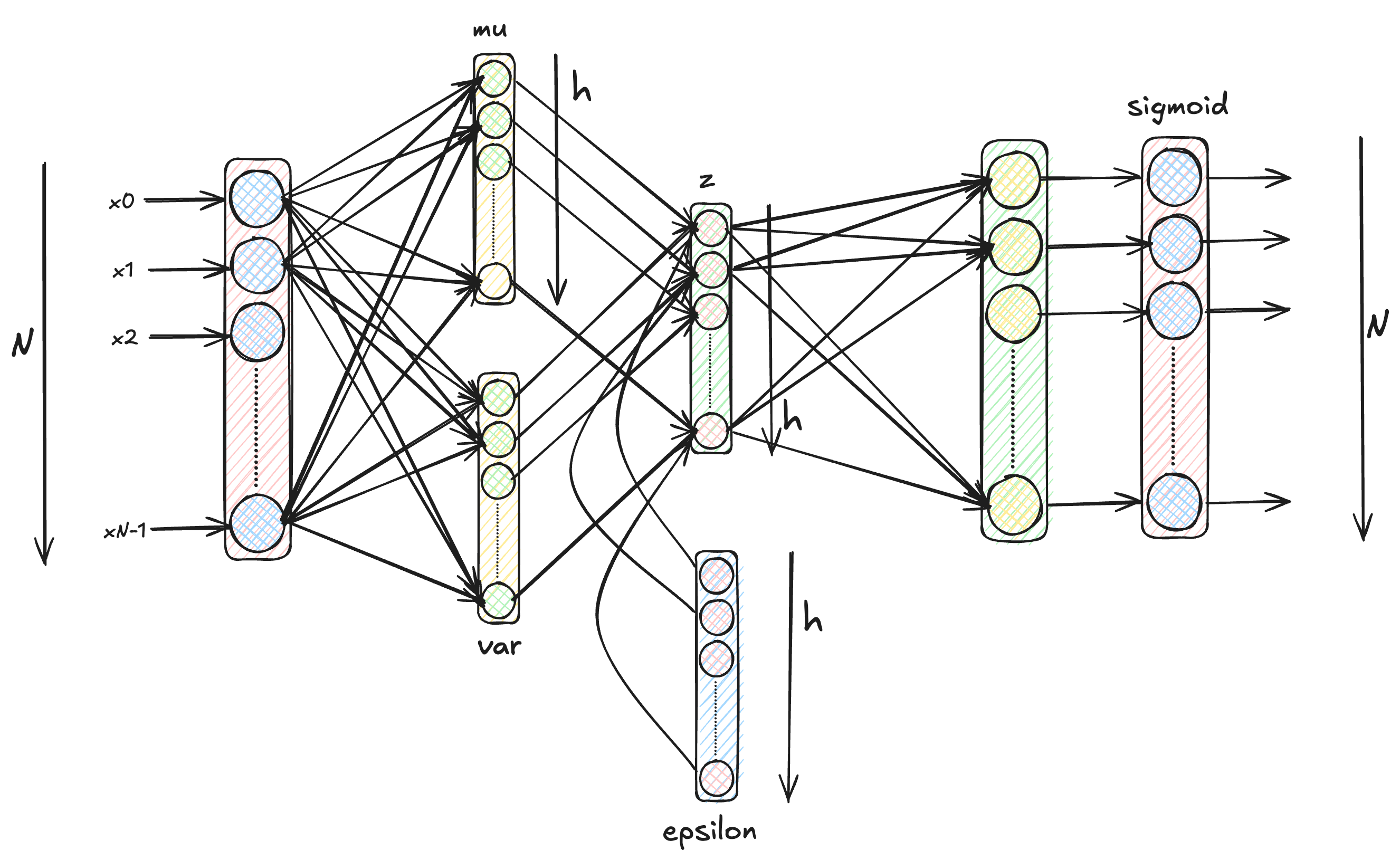
But before we deep dive into Variational Autoencoders, note that the problem statement is not to learn another neural network architecture. The problem we are trying to solve is a conditional probability estimation problem. We want to find the probability distribution of the latent space z given the inputs x i.e. p(z|x). This is essentially what we want to solve in the remainder of the post. The neural network architecture for VAE shown above is just the tool to achieve our goal of solving the probability estimation problem.

Using Bayes’ Theorem to compute the conditional probability of z given x as follows:



But the integral in the denominator is difficult to compute since it is over all possible latent states z. One possible way is to use sampling. Assuming normal distributions for both p(z) and p(x|z), we can sample few values of z and use them to approximate the integral in the denominator. But with few samples it will not give correct estimation.

Instead of computing p(z|x;theta) using the Bayes’ Theorem as above, we use some known and easy to compute probability distribution q(z|x;phi) as a proxy and then we minimize the difference between p(z|x;theta) and q(z|x;phi). Note that it is not necessary for p(z|x;theta) and q(z|x;phi) to be from the same family of distribution.

The difference between the probability distributions p(z|x,theta) and q(z|x,phi) can be captured using the KL Divergence as follows:



The last inequality implies that the log likelihood of p(x) has a lower bound known as ELBO (Evidence Lower Bound) which implies that maximizing the ELBO will also maximize the likelihood of p(x).

Recall that learning the parameters of a probability distribution is equivalent to maximizing the log likelihood (Maximum Likelihood Estimation) w.r.t. the parameters. The loss function for learning such a problem is usually the negative log likelihood (NLL). For eg. assuming that the output is normally distributed with a constant variance, the NLL of the normal distribution would look like:



Observe that the problem of estimating the probability distribution p(z|x;theta) has been transformed into an Expectation-Maximization(EM) problem. The expectation or the E step corresponds to estimating the expectation of the log likelihood i.e. E[ln(p(x;phi, gamma))] using the parameters phi and gamma. The maximization or M-step corresponds to maximizing the expectation i.e. max E[ln(p(x;phi, gamma))] and updating the values of the parameters phi and gamma.

Using a neural network with phi and gamma as weights, we can find the expectation value in the forward pass and do the maximization step in the loss calculation and backpropagation step. We saw the E-step above. Next we will see the M-step.

As mentioned earlier, we don’t need q(z|x;phi) to be of the same family as the original distribution of z, which means we can assume q(z|x;phi) to be normal distribution N(z;mu, var) where mu and var are the mean and variance of the normal distribution and these parameters are learnt using a neural network. Note that during actual training, we do not directly sample z from q instead we sample from a constant distribution epsilon ~ N(0,1) and then re-parameterize z as z=mu + epsilon*var which is same as sampling from N(mu, var). This is also known as the reparameterization trick and it allows gradients to flow backwards.

The KL divergence term can be expanded as follows:



Note that z, mu and var are h-dimensional vectors/tensors. We assume that each dimension of the latent space z is independently sampled from the probability distribution q(z|x). It is not apparent how the expectation terms are derived in the above derivation. We can show the proof of how the expectation terms are derived as follows:





We have derived the expression for the KL divergence term in the ELBO equation above pertaining to the log likelihood of p(x). Thus the substitited equation looks like below:



Coming to the next part of the equation, E[log(p(x|z;gamma)] i.e. the expectation of the log likelihood of the output given the latent state z. If we assume a normal distribution with a constant variance, then the log likelihood translates into MSE loss function whereas if we assume a Bernoulli distribution, then the log likelihood translates into Binary Cross Entropy (BCE) loss function.



If we do not assume a constant variance in the above equation, then we have another parameter to learn and the log likelihood function should be accordingly modified as follows:



The above term is assuming a normal distribution wherease the below term is assuming a bernoulli distribution.



Thus the loss function to learn for training the variational autoencoder is the negative log likelihood of p(x), which is as follows (for BCE loss):