Practical lessons learnt from building a demand-supply forecasting model

Sometimes back, I was leading a project at Microsoft to build their demand and supply forecasting models for spot virtual machines running in Azure. The idea behind using the demand-supply forecast models is to improve the dynamic pricing algorithm for spot instances.

For people who are unaware of spot virtual machines, almost all cloud service providers provide them. These virtual machines comes at a discounted price compared to the standard virtual machines (roughly 10% to 90% discount) but with the gotcha that these spot VMs can be evicted (read: Job killed) anytime depending on the current demand and bids. (Think like an auction).

An optimal pricing algorithm for these spot instances should take into account the projected demand and supply because we do not want to price these VMs too less such that the demand for these exceeds the projected supply. The exact dynamic pricing algorithm is a story for another post though.

The demand-supply forecasting deals with 700+ different virtual machines e.g. standard_d16s_v5, running across 100+ regions and running either linux or windows OS. Thus, there are approx. 700 * 100 * 2 = 140K different time series for demand as well as supply or 280K in total considering both demand and supply together.

Each time series uses last 365 days worth of data i.e. approximately 102M values.

Some lessons learnt and choices made while taking this project to completion:

Using deep learning models from the word go instead of spending time on classical ML techniques such as ARIMA, Gradient Boosting for forecasting etc.

That is not to say that classical forecasting algorithms and gradient boosting are not good algorithms. From our experience working with forecasting problems in similar domains, we have found that deep learning models often outperform ARIMA or XGBOOST and also we save time on manually creating features such as finding the periodicity using Fast Fourier Transforms etc.

Another reason is that the predictions from our forecasting models are not consumed in real time, and thus we took the liberty to improve the accuracy of the forecasts. Regression models are faster with inference times but performs poorly as compared to deep learning models.
Modelling all the 280K time series together instead of individually modelling them or creating sub-groups based on VM or region or OS etc.

The advantages of a single model over multiple models are as follows:

a. A significant number of (VM, region and OS) tuples have very less data and thus modelling them separately do not make much sense.

b. Ease of maintenance. It is easier to build and maintain a single model.

c. Better with cold start problem. New VMs will not have enough time series data.
Using distributed map-reduce jobs wherever feasible to deal with large datasets and to reduce data processing times. But understanding where map-reduce will be beneficial vs. wherever not.

Running map-reduce over distributed nodes has an additional network overhead due to multiple I/Os over the network. The problem can be significant if the executor nodes are located very far away from the driver node or some executor nodes is crashing occassionally and the scheduler has to retry the task. This is advantageous when:

a. Driver node has limited memory and cannot run with all data at once.

b. Driver node has enough memory but CPU time taken is more as compared to solving it in parallel + network overhead.

Map-reduce template with Pyspark:
```
 def mapr(objects):
   def evaluate(object):
     result = do_something(object)
     return result

   rdd = spark.sparkContext.parallelize(objects, len(objects))
   out = rdd.map(evaluate)
   res = out.collect()
```
Use static features corresponding to virtual machines in addition to other time dependent features.

Static features and other time dependent features apart from the time series values helps to distinguish different time series i.e. different (VM, region, OS) tuples without actually using categorical variables to identify these.

The advantage is that if some new (VM, region, OS) tuple is added after the model is built, we can still get predictions using the last 30 days data.

If we had used categorical feature to identify the tuple, we cannot get predictions from the trained model because the model has not seen those features.

Some examples of generic static features are number of CPU cores in a VM, RAM and SSD sizes, set of hardwares where the VM can run and so on.
Instead of auto-regressive model, we chose to use a multi-horizon forecast model.

In auto-regressive model, we feed the prediction of day D as input to the network to generate prediction for day D+1 and so on. Thus to predict the demand forecast for day D+29, it would use last 29 days of predicted values and only 1 actual value.

If each prediction has some error, then the errors will accumulate over all the 29 days. Instead we prefer to use a multi-horizon model where the model predicts the forecasts for days D to D+29 in one-shot using only the actual values D-30 to D-1.

Multi-horizon models gave better metrics on MAPE and MSE values as compared to auto-regressive models.
Using efficient data compression and time series compression algorithms as well as sparse data structures for distributed map-reduce jobs reduces processing times as well as memory usage.

One of the tricky parts during the map-reduce operations is that the task results from each executor node could be well over few 100 GBs. Sending all the data over the network could consume significant network bandwidth and could be very slow.

Moreover, the driver node that is collecting all the data from multiple executors will be holding M*100 GB of data where M is the number of executor nodes. This could easily go out-of-memory.

One possible way to reduce of the size of the data transferred is to use compression. Some strategies that we felt are useful for compressing the data:

a. If the result is a sparse NumPy matrix, then use scipy.sparse.csr_matrix format instead of numpy.array().

b. If the result are time series values, then encode each time series separately using delta encoding or XOR encoding techniques. Gorilla paper from Meta is a nice reference on how to do XOR encoding of time series data.

c. If the data is a dense matrix, then one can use histogram based encoding for each floating point columns. Note that these are lossy encoding and are useful only if you are going to use the histogram encoding as features to your model.

d. Another lossy encoding is to do dimensionality reduction using Truncated SVD or PCA. Again this is useful only when the encoded columns are being used as features to the model.

If all else fails, and you are still getting out-of-memory errors, one possible solution is to persist the resultant objects in a blob storage container and read them back from storage sequentially.
Using Conv1D architectures instead of LSTM or RNN based deep learning models gives almost equivalent or better performances but much higher speed of training and inference.

Convolution operations such as Conv1D are nothing but multiple matrix dot product operations. Such operations can be easily parallelized across different regions of the matrix and each matrix dot product can leverage SIMD or GPU instructions for faster computations.

On the other hand LSTM and RNN are sequential architectures. They cannot be parallelized.

For our problem, Conv1D was at-least 8 times faster than LSTM architecture while giving similar results.
There are lots of missing data in the time series’. Handling missing data using exponential averaging improves the overall model performance.

Simple averaging of past N days values gives equal weightage to all the past N days but in a time series, usually the recent values are better predictor than the older values.

Thus, we chose to use an exponentially weighted average, where the value for day D-H is given a weightage of exp(-H/K). H is the number of days backwards from current day D and K is a constant e.g. 30.
```
 import numpy as np
 def exponential_averaging(values, index_to_fill, past_N, K=30):
    s = 0
    u = 0
    for i in range(index_to_fill-1, max(-1, index_to_fill-past_N-1), -1):
        h = np.exp(-(index_to_fill-i)/K)
        s += h*values[i]
        u += h
    values[index_to_fill] = s/u if u > 0 else 0.0
```
Encoding of categorical and numerical features efficiently so as not to explode the size of the matrices in memory as well as not sacrifice on performance.

Neural networks requires all input data to be numerical. Thus any categorical features such as region, OS etc. needs to be converted into numerical features. One strategy is using one-hot encoding. But with 700+ products, the size of a one-hot encoded vector would be 700+ with lots of zeros.

We did Truncated SVD on the sparse matrix to reduce dimensionality.

For numerical features (floats etc.) we had used binning strategy to encode the features. The number of bins to use can be chosen by hyperparameter tuning.

We had used the starting boundary value of each bin as encoded feature values.
Explicit garbage collections of large in-memory objects while working with notebooks, helps iterate faster with less resources.

While working with notebooks, if we do not take care, very quickly the size of the objects held in the memory would cause the notebook to crash with out-of-memory errors.

One strategy is to do explicit garbage collection of large objects in memory.

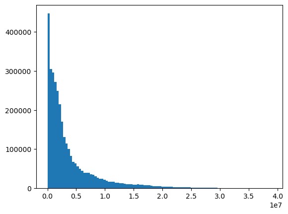
Another startegy is to persist large objects in the blob storage and read then back in another session or another job.

Demand and supply data do not follow a normal distribution but the data is highly skewed with a long tail resembling a Gamma or a Negative Binomial Distribution. Thus, care must be taken while defining the loss function.

Usual loss functions used in regression and time series forecasting are mean squared errors or mean absolute errors. But with skewed data, MSE or MAE may not be the best choice. Remember that the loss function is derived from the maximum likelihood principle of the distribution of the target variable. Usually we take the negative log likelihood.

MSE or MAE works best when we assume that the target variable follows a normal distribution.

In our case, our distribution for demand and supply follows a distrubtion similar to a Gamma or a Negative Binomial distribution.

In Tensorflow, we can define custom loss for a gamma distribution as follows:

def gamma_loss():
   def loss(y_true, y_pred):
       # k is the shape parameter > 0 and m is the mean of the gamma distribution
       k, m = tf.unstack(y_pred, num=2, axis=-1)
   
       k = tf.expand_dims(k, -1)
       m = tf.expand_dims(m, -1)
   
       l = tf.math.lgamma(k) + k*tf.math.log(m) - k*tf.math.log(k) - (k-1)*tf.math.log(y_true+1e-7) + y_true*k/y_pred
           
       return tf.reduce_mean(l)
   
   return loss

def negative_binomial_loss():
   def loss(y_true, y_pred):
       # r is the parameter for number of successes and m is the mean of the distribution
       r, m = tf.unstack(y_pred, num=2, axis=-1)
   
       r = tf.expand_dims(r, -1)
       m = tf.expand_dims(m, -1)
   
       nll = (
           tf.math.lgamma(r) 
           + tf.math.lgamma(y_true + 1)
           - tf.math.lgamma(r + y_true)
           - r * tf.math.log(r) 
           + r * tf.math.log(r+m)
           - y_true * tf.math.log(m) 
           + y_true * tf.math.log(r+m)
       )
   
       return tf.reduce_mean(nll)       
       
   return loss

Supply Data Distribution

Probabilistic forecasting model to handle different quantiles at once instead of a single quantile regression model.

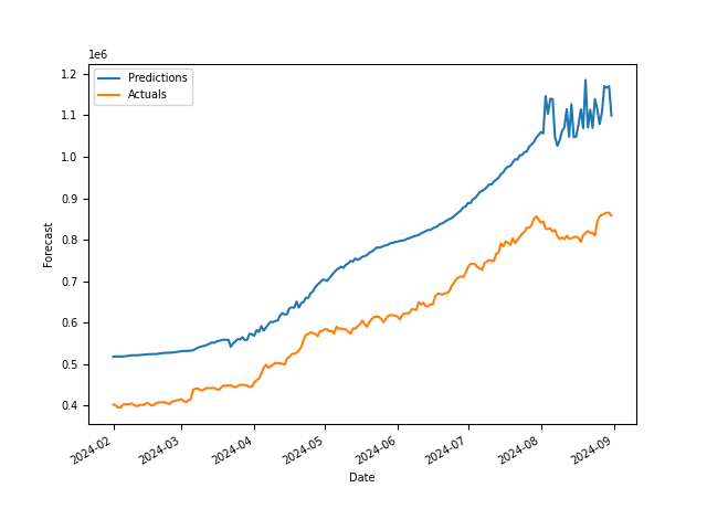
Instead of only predicting the mean of the distribution of the demand and supply as forecasted values, our network also predicts the parameters of the distribution. This has the advantage that we can use the distribution to predict different quantiles for the demand and supply forecast values. For e.g. 90% quantile implies that the predicted values are greater than the true values 90% of the time.

For VM forecasting, we want to make sure that there is always sufficient buffer capacity available in case demand peaks, P90 or P99 forecast values can be useful here.

P99 Demand Forecast results for one (VM, Region, OS) pair:

Using memory mapped files or hdf5 to store and read large NumPy arrays.

The size of the entire training matrix was approx. 800GB in size. Working with such large arrays would definitely cause out-of-memory errors on nodes with 64GB RAM. To train a Tensorflow model without loading the entire data in memory, we first write the array to disk using memory mapped files. Then read them back with shuffled indices from disk in batches.

Shuffling is done so that during training of the model, each batch contains a good-mix of different (VM, Region, OS) tuples. Reading is done using a custom generator function. Load the memory mapped file and read and generate the batches for training the model.

But note that memory mapped file works only with local filesystems. In Azure, we mount the blob storage to Spark clusters and thus we can work with blob storage as if it were a local filesystem.

import numpy as np
    
# write to file on disk
fpx = np.memmap("xdata.npy", dtype='float64', mode='w+', shape=(n,t,m))
fpx[:,:,:] = X[:,:,:]
fpx.flush()

fpy = np.memmap("ydata.npy", dtype='float64', mode='w+', shape=(n,t,m))
fpy[:,:,:] = Y[:,:,:]
fpy.flush()

def datagen(batch_size):
   fpx = np.memmap("xdata.npy", dtype='float64', mode='r', shape=(n,t,m))
   fpy = np.memmap("ydata.npy", dtype='float64', mode='r', shape=(n,t,m))

   # shuffle data
   shuffled = np.random.shuffle(np.arange(n))
   indices = list(np.arange(n))
    
   start = 0
    
   while True:
      end = min(n, start+batch_size)
      batch = indices[start:end]
   
      x = fpx[batch,:,:]
      y = fpy[batch,:,:]

      start += batch_size
   
      if start >= n:
         start = 0
   
      yield x, y

Feature scaling led to very small floating point numbers for demand and supply leading to vanishing gradient problem famously associated with deep neural networks. Care must be taken so as not to scale down features which are already very small.

Using MinMaxScaler() to scale the values for demand and supply led to very small values because the actual range was 1 to 1e7, and after scaling, the range shifted to 1e-7 to 1.

During backpropagation, the feature values are multiplied with the gradient to obtain the updated weights. If both gradient and feature values are very small, then the weight updates are negligible and the network does not train properly.

Better strategy was not to scale the demand and supply values as both these time series were of similar scales.
Using int32 instead of float64 for demand and supply values reduced memory consumption.

Demand and supply values are usually in terms of number of virtual cores of a VM and number of vcores are usually integers. Using int32 (32-bit) data type instead of float64 (64-bit) reduced memory consumption.
Choosing the offline metrics wisely. Just don’t (only) use MAPE.

MSE or MAE for offline evaluation were not meaningful for us, as for large demand and supply values, the error can also be large. For e.g. an error of 1000 on 10000 is better than an error of 10 on 20.

This calls for using MAPE (Mean Absolute Percentage Error). Thus instead of absolute difference, we take the percentage change which in the above example is 10% for the former and 50% for the latter.

But a MAPE can also be deceiving. For e.g. for an actual value of 1000, a prediction of 2000 and a prediction of 0 will both have the same MAPE but a prediction of 2000 is much more acceptable than 0 which could have happened due to underfitting or overfitting of the model.

Another metric could be the quantile (pinball) loss if we are using quantile forecasting.

A single metric may not be an ideal solution for this problem.

Pinball Metric:
```
def pinball_loss(quantile, y_true, y_pred):
   e = y_true - y_pred
   return np.mean(quantile*np.maximum(e, 0) + (1-quantile)*np.maximum(-e, 0))
```

Sample Architecture for demand and supply forecasting:

The input demand-supply time series is a 3D Tensor with a shape of (N, 30, 1) where N is the batch size and 30 is the number of time-steps. Thus, we are inputting 2 time series’ and outputting 2 time series’.

def gamma_layer(x):
    num_dims = len(x.get_shape())

    k, m = tf.unstack(x, num=2, axis=-1)

    k = tf.expand_dims(k, -1)
    m = tf.expand_dims(m, -1)

    # adding small epsilon so that log or lgamma functions do not produce nans in loss function
    k = tf.keras.activations.softplus(m)+1e-3
    m = tf.keras.activations.softplus(m)+1e-3
 
    out_tensor = tf.concat((k, m), axis=num_dims-1)
 
    return out_tensor

def gamma_loss():
    def loss(y_true, y_pred):
        k, m = tf.unstack(y_pred, num=2, axis=-1)

        k = tf.expand_dims(k, -1)
        m = tf.expand_dims(m, -1)

        l = tf.math.lgamma(k) + k*tf.math.log(m) - k*tf.math.log(k) - (k-1)*tf.math.log(y_true+1e-7) + y_true*k/y_pred
        
        return tf.reduce_mean(l)

    return loss

class ProbabilisticModel():
    def __init__(
        self, 
        epochs=200, 
        batch_size=512, 
        model_path=None,
        use_generator=True
    ):
        self.epochs = epochs
        self.batch_size = batch_size
        self.model_path = model_path

    def initialize(self, inp_shape_t, inp_shape_s, out_shape):

        # inp_shape_t - shape of the input demand-supply time series
        # inp_shape_s - shape of the input static features
        # out_shape   - shape of the output demand-supply time series

        inp_t_dem = Input(shape=inp_shape_t)
        inp_t_sup = Input(shape=inp_shape_t)

        inp_s = Input(shape=inp_shape_s)

        x_t = \
            Conv1D(
                filters=16, 
                kernel_size=inp_shape_t[0], 
                activation='relu', 
                input_shape=inp_shape_t
            )
                
        x_h = Dense(16, activation='relu')
        
        x_dem = x_h(x_t(inp_t_dem))
        x_sup = x_h(x_t(inp_t_sup))

        x_s = Dense(8, activation='relu')(inp_s)

        x_s_dem = Concatenate()([x_s, x_dem])
        x_s_sup = Concatenate()([x_s, x_sup])

        out_dem = Dense(out_shape[0]*2)(x_s_dem)
        out_dem = Reshape((out_shape[0], 2))(out_dem)
        out_dem = tf.keras.layers.Lambda(gamma_layer)(out_dem)

        out_sup = Dense(out_shape[0]*2)(x_s_sup)
        out_sup = Reshape((out_shape[0], 2))(out_sup)
        out_sup = tf.keras.layers.Lambda(gamma_layer)(out_sup)
                
        self.model = Model([inp_t_dem, inp_t_sup, inp_s], [out_dem, out_sup])
        
        self.model.compile(
            loss=[gamma_loss(), gamma_loss()], loss_weights=[1.0, 1.0], 
            optimizer=tf.keras.optimizers.Adam(0.001)
        )
    
    def fit(self, X_t_dem:np.array, X_t_sup:np.array, X_s:np.array, y_dem:np.array, y_sup:np.array):

         # X_t_dem - input demand time series
         # X_t_sup - input supply time series
         # X_s     - input static features
         # y_dem   - output demand time series
         # y_sup   - output supply time series

         model_checkpoint_callback = \
            tf.keras.callbacks.ModelCheckpoint(
                filepath=self.model_path,
                monitor='loss',
                mode='min',
                save_best_only=True
            )
        
         self.model.fit\
            (
                [X_t_dem, X_t_sup, X_s], [y_dem, y_sup], 
                epochs=self.epochs, 
                batch_size=self.batch_size, 
                validation_split=None, 
                verbose=1, 
                shuffle=True,
                callbacks=[model_checkpoint_callback]
            )
    
    def predict(self, X_t_dem:np.array, X_t_sup:np.array, X_s:np.array):
        return self.model.predict([X_t_dem, X_t_sup, X_s])
    
    def save(self):
        self.model.save(self.model_path)
    
    def load(self):
        self.model = \
            load_model(
                self.model_path, 
                custom_objects={
                    'gamma_layer':gamma_layer,
                    'loss':gamma_loss()
                })

Sample Architecture for demand and supply forecasting:

Suggested Readings