Experimenting with time series floating point compression
While working on time series forecasting for demand and supply of spot virtual machines in Azure, intermediate data processing was done in a distributed fashion using Spark. Often the data size in each executor node exceeded 50-100 GB. This caused some issues while doing map-reduce operations.
-
When the results from each executor node was collected at the driver node, the data size
exceeded available RAMand caused the driver nodes to crash. -
Transferring GBs of data over network has
throughput implications. Network transfers of large data often took long time.
One hack we did early on to mitigate issue number 1 above was to write the outputs of the executor nodes into blob storage in Azure. Then read back the files from the driver node sequentially and process the data without hogging a lot of memory. Once we mounted the blob storage using NFS, reading and writing became a lot faster.
For issue number 2, there was no fast hack but to compress the outputs of each executor node before sending them over the network. Sometimes the data structure was a dataframe with mixed data types, sometimes it was just a NumPy matrix. But most often they were time series data.
One very interesting property of time series data is that consecutive values in a time series are often closer to one another. But it does not imply that values that are far-apart are not close to one another. Most contemporary time series compression algorithms take advantage of this fact while coming up with a compression algorithm.
In this post, I will only show how to compress time series with floating point numbers instead of generalizing to integers and timestamps. While it is easier to compress integer values in a time series using either delta encoding or dictionary encoding, these strategies do not work with floating points because, difference of 2 64-bit floats is still a 64-bit float while a difference between 2 64-bit ints can even be a 8-bit int if the values are close to one another.
Or, if there are very few unique integer values one can also use dictionary encoding. On the other hand, floats are “infinite”.
Common floating point compression algorithm assumes that floats that are closer to one another in terms of absolute values, are also closer to one another in terms of their binary representations.
While this might hold true in certain cases but in general this is not true.
But anyways, our focus for this post will be on XOR compression, which works on this assumption.
But first lets understand how floating point numbers are represented in binary. We will take the example of 64-bit floats as this was the most commonly used format in our work.
The 1st bit is the sign bit - 0 for +ve and 1 for -ve.
The next 11 bits represent the exponent.
The remaining 52 bits are called the significand or mantissa.
For e.g. if N=316.9845
- Represent the number in binary. For e.g. 316 is represented in binary as 100111100. The fraction 0.9845 can be converted to binary by repeatedly multiplying by 2 and taking the integer part out.
0.9845 * 2 = 1.9690 - Take out 1
0.9690 * 2 = 1.9380 - Take out 1
0.9380 * 2 = 1.8760 - Take out 1
....and so on.
Finally we get the binary for 0.9845 as 11111100000010000011000100100110111010010111100011011
Representing 316.9845 in binary, we have:
X=100111100.11111100000010000011000100100110111010010111100011011 -
Next, write the representation in 1.xxxxx format i.e.
X=1.0011110011111100000010000011000100100110111010010111100011011 * 2^8For 64 bits, the power of 2, is usually written as 1023+p. Here p=8, thus we have
X=1.0011110011111100000010000011000100100110111010010111100011011 * 2^(1031-1023) -
The binary representation of the exponent 1031 is 10000000111. The final representation is the concatenation of the following:
a. 0 bit because the number is +ve
b. Binary representation of 1031 (the exponent) : 10000000111
c. The first 52 bits after the decimal point in the above representation i.e. 0011110011111100000010000011000100100110111010010111The final representation is : 0100000001110011110011111100000010000011000100100110111010010111
Since we have taken 52 relevant bits out of 61 bits, the final representation is rounded: 0100000001110011110011111100000010000011000100100110111010011000
In Python, we can get the 64 bit representation from a float as follows:
import bitstring
def float_to_bin(x):
  f = bitstring.BitArray(float=x, length=64)
  return str(f.bin)
Similarly, we can obtain the floating point value from a 64-bit representation as follows:
For e.g. given the following pattern:
X = 0100000001011110110001111101111100111011011001000101101000011101
- The 1st bit is 0 indicating it is a +ve number.
- The next 11 bits are : 1000000010 represents 1029. Subtracting off 1023 gives us 6. Thus the exponent is 2^6.
- The remaining bits are 1110110001111101111100111011011001000101101000011101. Thus the decimal format is (adding 1. before it): 1.1110110001111101111100111011011001000101101000011101
Thus we have the number:
X = 1.1110110001111101111100111011011001000101101000011101 * 2^6, or
X = 1111011.0001111101111100111011011001000101101000011101.
The integer part is 1111011 or 123.
The fractional part is 0001111101111100111011011001000101101000011101.
To get the base-10 of the fractional part, for each bit at position i we multiply it by 2^(-(i+1)). We get the base-10 of the fractional part as 0.12300000000000466.
def get_integer_from_binary_fraction(s):
  c = 0
  for i in range(len(s)):
      c += 2**(-(i+1)) if s[i] == '1' else 0
  return c

get_integer_from_binary_fraction('0001111101111100111011011001000101101000011101')
# 0.12300000000000466
Thus, the final value is 123.123 (rounded).
In Python, one can obtain the floating point value from a 64-bit representation as follows:
import struct
def bin_to_float(binary):
    return struct.unpack('d', struct.pack('Q', int(f'0b{binary}', 0)))[0]
Now let’s turn our attention to XOR Compression.
Assuming that in a time series consecutive values are closer to one another and their binary representations are also close (not true in general), then there will be many bits common between consecutive 64 bit representations. Thus, if we take the XOR of consecutive values, then there will be lots of zeros.
T   - 10110111000...110
T+1 - 10010111110...010

XOR - 00100000110...100
We implemented a simple version of the algorithm outlined in the Gorilla paper from Meta. But in order to handle the scenario where the binary representations for consecutive values are not similar, we implemented a modified version (specifically TSXor) that compares the current value with all values within a sliding window of size N.
import bitstring, struct
from collections import deque
import numpy as np

def compress(ser, log_window=4):
    # store the sliding window of historical 64-bit representations
    prev_bins = deque([])
    results = []

    for i in range(len(ser)):
        x = ser[i]
        b = float_to_bin(x)

        # p - index of 1st '1' from the left
        # q - index of 1st '1' from the right
        # q-p+1 - length of the relevant block

        p, q = -1, -1
        r, y = '', ''

        if i == 0:
            y = b
            r = b

            for j in range(len(b)):
                if b[j] == '1':
                    p = j
                    break

            for j in range(len(b)-1, -1, -1):
                if b[j] == '1':
                    q = j
                    break

        else:
            v = 0
            min_dist = float("Inf")
            best_p, best_q = -1, -1
            best_xor = ''
            best_res = ''

            for h, pp, pq, px in prev_bins:
                p, q = -1, -1

                # y - XOR of b (current) and h (historical)
                y = ''
                for j in range(len(b)):
                    y += '1' if b[j] != h[j] else '0'

                for j in range(len(y)):
                    if y[j] == '1':
                        p = j
                        break

                for j in range(len(y)-1, -1, -1):
                    if y[j] == '1':
                        q = j
                        break

                if p == -1:
                    # No '1' found in XOR implies b is same as some h
                    r = '0'
                    d = 1
                else:
                    f = 1
                    # Relevant block is a sub-block of some historical value
                    if p >= pp and q <= pq:
                        is_sub = True
                        for j in range(p, q+1):
                            if y[j] != px[j]:
                                is_sub = False
                                break

                        if is_sub:
                            f = 0

                    # 6 bits to store starting index p (0-63)
                    k = bin(p)[2:]
                    k = '0'*(6-len(k)) + k

                    # 6 bits to store ending index q (0-63)
                    g = bin(q)[2:]
                    g = '0'*(6-len(g)) + g

                    # log_window bits to store index of most similar representation
                    z = bin(len(prev_bins)-v-1)[2:]
                    z = '0'*(log_window-len(z)) + z

                    if f == 0:
                        r = '10' + z + k + g
                    else:
                        r = '11' + z + k + g + y[p:q+1]

                    d = len(r)

                if d < min_dist:
                    min_dist = d
                    best_p = p
                    best_q = q
                    best_xor = y
                    best_res = r

                v += 1

            r = best_res
            p = best_p
            q = best_q
            y = best_xor

        results += [r]
        prev_bins.append((b, p, q, y))
        if len(prev_bins) > (1<<log_window):
            prev_bins.popleft()

    # pad with 0s to make multiple of 8
    s = ''.join(results)
    n = len(s)
    m = n%8
    m = 8 if m == 0 else m
    s += '0'*(8-m)

    # Convert the bits into bytes
    res = []
    for i in range(0, len(s), 8):
        g = int(s[i:i+8], 2)
        res += [g]

    return np.array(res).astype('uint8'), n
The compression algorithm is as follows:
- For the 1st value, store the 64-bit representation as is.
- For the i-th value (i > 1), calculate the 64-bit representation, then find the
XORvalue with each of the representations in the sliding window. - The sliding window size defined above is 16 i.e. the current 64-bit representation is compared with the previous 16 representations.
- For each of the 16 representations in the sliding window, the XOR value between j and i is computed where i - current representation, j - one of the 16 representations in sliding window.
-
The XOR that gives the best reduction in size is kept. The resultant representation after XOR is either of the following:
a.'0'- if the XOR is 0 for all 64 bits.
b.'10'+4-bitsfor the index of themost similar representationw.r.t. current index in the sliding window +6-bitsfor thefirst index of 1 bitin the XOR representation +6-bitsfor thelast index of 1 bitin the XOR representation.
c.'11'+ 4-bits for the index of the most similar representation w.r.t. current index in the sliding window + 6-bits for the first index of 1 bit in the XOR representation + 6-bits for the last index of 1 bit in the XOR representation + XOR representation between the first index of 1 bit and last index of 1 bit.For e.g. if the current representation at index 25 is:
X = 0100000001011110110001111101111100111011001001000101100011010001
and the representation at index 19 is:
Y = 0100000001011110110001111101111100111011011001000101101000011101
Then the XOR is:
Z = 0000000000000000000000000000000000000000010000000000001011001100Then the first index of 1 bit in Z is 41 and last index is 61. 4-bits for the index of Y is binary(25-19-1=5) = 0101 6-bits for first index of 1 i.e. 41 = 101001 6-bits for last index of 1 i.e. 61 = 111101The control bits ‘0’, ‘10’ and ‘11’ are prefix-disjoint meaning that neither is a prefix of any other.
Since the XOR Z does not have all ‘0’, the representation will be either ‘10’ or ‘11’.
‘10’ is chosen when the XOR at index 25 is a ‘sub-XOR’ of the XOR at index 19, i.e. the first and last index of 1 at index 25 lies in-between the first and last index of 1 of the XOR at index 19 and the XOR at index 25 between the first and last index of 1 is equal to the XOR between the first and last index of 1 at index 19.
If this is the case then we do not need to explicitly store the XOR value between the first and last index of 1 because once we know the XOR at index 19, we can infer the XOR at 25 given the first and last index of 1 at index 25.
Else, we use the option ‘c’ with control bits ‘11’. Concatenateall the compressed binary representations from all values in the time series.- Convert them to
8-bit integervalues and return the compressed array.
To compute the compression ratio, we can do with something like:
import sys
import numpy as np

a = np.random.normal(100.0,0.1,10000)
g, n = compress(a)
# n - size of compressed binary

print("Compression ratio = ", 1.0 - sys.getsizeof(g)/sys.getsizeof(a))
To decompress the compressed values, I used the following Python function:
def decompress(arr, n, log_window=4):
    # Convert 8-bit integers to binary and concatenate them
    bins = []
    for i in range(len(arr)):
        x = arr[i]
        b = str(bin(x)[2:])
        b = '0'*(8-len(b)) + b
        bins += [b]

    s = ''.join(bins)
    s = s[:n]

    results = []
    prev_xors = deque([])

    i = 0
    while i < len(s):
        if i == 0:
            # First value is as is (not compressed)
            results += [s[i:i+64]]
            prev_xors.append([s[i:i+64]])
            i += 64

        else:
            # Parse the binary string to decompress
            if s[i] == '0':
                results += [results[-1]]
                prev_xors.append(['0'*64])
                i += 1

            else:
                # Get the relative index of the most similar binary representation
                z = int(s[i+2:i+2+log_window], 2)

                # Get the first index of 1 in its XOR
                p = int(s[i+2+log_window:i+8+log_window], 2)

                # Get the last index of 1 in its XOR
                q = int(s[i+8+log_window:i+14+log_window], 2)

                if s[i:i+2] == '10':
                    # Get the XOR for most similar entry
                    assert z+1 <= len(prev_xors), "Incorrect compression !!!"
                    y = prev_xors[-(z+1)]

                    u = ['0']*64

                    # Substitute the XOR of most similar entry in [p, q]
                    u[p:q+1] = y[p:q+1]

                    # Do XOR to get back the original entry. XOR'ing twice gives back the original value.
                    v = results[-(z+1)]
                    f = ''
                    for j in range(len(u)):
                        f += '1' if u[j] != v[j] else '0'

                    results += [f]
                    prev_xors.append([''.join(u)])
                    i += 14+log_window

                else:
                    # Get the relevant bits in the XOR
                    y = s[i+14+log_window:i+14+log_window+q-p+1]

                    u = ['0']*64

                    # Substitute the XOR in [p, q]
                    u[p:q+1] = y

                    # Do XOR to get back the original entry. XOR'ing twice gives back the original value.
                    v = results[-(z+1)]
                    f = ''
                    for j in range(len(u)):
                        f += '1' if u[j] != v[j] else '0'

                    results += [f]
                    prev_xors.append([''.join(u)])
                    i += 14+log_window+q-p+1

        if len(prev_xors) > (1 << log_window):
            prev_xors.popleft()

    # Convert the binary representations to floats
    results = [bin_to_float(x) for x in results]

    return np.array(results).astype('float64')

b = decompress(g, n)
assert sum(a != b) == 0, "Compression and decompression mismatch !!!"
Depending on how big a sliding window we use, we trade-off compression/decompression time and space complexity in favor of better compression ratios. But usually increasing the sliding window to very large values has diminishing returns.
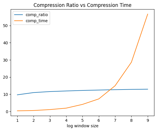
I ran the above experiments using values sampled from a random normal distribution (100, 0.1) and the compression ratios varied somewhere from 9% to 14% with window sizes ranging from 1 to 10. Increasing window sizes definitely improved the compression ratio but at the cost of high compression times. The compression ratio also improves if the standard deviation for the normal distribution is small implying that when values are more closer to each other, they have more similar binary representations.
Real world datasets can have arbitrary distributions. Some real world distributions can give very good compression ratios like 50% or 70% etc. But some datasets can give very bad compressions too. One problem with the above compression algorithm is that the average number of bits required to compress a 64-bit binary value can be greater than 64 if the XOR has lots of 1s in it.
I tried using ML in the hope to find better compression ratios. The idea goes like this:
- For compressing the i-th value, build a
time series forecasting modelusing inputs from i-1 to i-N. Use this model to predict the i-th value.
The inputs and outputs are the 64-bit binary representations instead of actual values. Thus the inputs and output are64 dimensional vectorsof 1s and 0s. - Instead of taking XOR with all values in a sliding window, take XOR between the actual i-th value and the predicted i-th value. Thus, if the model is good, the predicted value would be close to the actual value and thus more number of 0s in the XOR.
- Similarly, during decompression, using the last N predicted values, predict the i-th value and take an XOR with the decompressed XOR value for the i-th entry.
Python codes to create the time-series forecasting data for a deep learning model.
import numpy as np
def create_ts(seq, lookback=30, future=1):
    X, Y = [], []
    bin_seq = []
    for i in range(len(seq)):
        x = seq[i]
        b = float_to_bin(x)
        b = [int(z) for z in list(b)]

        # Convert 64-bit binary string into 64 size int vector
        bin_seq += [b]

    for i in range(len(bin_seq)-lookback-future+1):
        xi = bin_seq[i:i+lookback]
        yi = bin_seq[i+lookback:i+lookback+future]
        X += [xi]
        Y += [yi]

    X = np.array(X)
    Y = np.array(Y)

    return X, Y
The deep learning model architecture is kept simple using a Conv1D layer, a dense ReLU layer and an output layer with 64 units each emitting a value between 0 and 1 using a sigmoid activation. Thus if the predicted value is <= 0.5, then we consider it as 0 else we consider it as 1.
class TSModel():
    def __init__(
        self,
        epochs=200,
        batch_size=512,
        model_path=None
    ):
        self.epochs = epochs
        self.batch_size = batch_size
        self.model_path = model_path

    def initialize(self, inp_shape, out_shape):
        inp = Input(shape=inp_shape)

        # 1-D Convolution wth kernel size equals to 30.
        x_t = \
            Conv1D(
                filters=256,
                kernel_size=inp_shape[0],
                activation='relu',
                input_shape=inp_shape
            )(inp)

        # Dense layer with ReLU activation
        x_t = Dense(128, activation='relu')(x_t)

        # OUtput layer with 64 units and sigmoid activation. Each unit will produce a value between 0 and 1
        out = Dense(out_shape[1], activation='sigmoid')(x_t)

        self.model = Model(inp, out)

        self.model.compile(
            loss='binary_crossentropy',
            optimizer=tf.keras.optimizers.Adam(0.001)
        )

    def fit(self, X:np.array, Y:np.array):
        # Save model using checkpointing
        model_checkpoint_callback = \
            tf.keras.callbacks.ModelCheckpoint(
                filepath=self.model_path,
                monitor='loss',
                mode='min',
                save_best_only=True
            )

        self.model.fit\
        (
            X, Y,
            epochs=self.epochs,
            batch_size=self.batch_size,
            validation_split=None,
            verbose=1,
            shuffle=True,
            callbacks=[model_checkpoint_callback]
        )

    def predict(self, X:np.array):
        return self.model.predict(X)

    def save(self):
        self.model.save(self.model_path)

    def load(self):
        self.model = \
            load_model(self.model_path)
The corresponding compression and decompression algorithms are:
# compression
def compress_ml(ser, model, lookback=30):
    results = []

    # generate the predictions on the same dataset
    X, _ = create_ts(ser)
    preds = model.predict(X)
    predsl = []

    for pred in preds:
        pr = pred[0]

        # Label is 1 if model prediction is > 0.5 else 0
        pr = ['1' if zz > 0.5 else '0' for zz in pr]
        h = ''.join(pr)
        predsl += [h]

    for i in range(len(ser)):
        x = ser[i]
        b = float_to_bin(x)

        p, q = -1, -1
        r, y = '', ''

        if i < lookback:
            # No compression for the 1st 30 values
            r = b
        else:
            p, q = -1, -1
            h = predsl[i-lookback]

            # Get the XOR between actual binary rep and predicted binary rep
            y = ''
            for j in range(len(b)):
                y += '1' if b[j] != h[j] else '0'

            # Get the first index of 1 in the XOR
            for j in range(len(y)):
                if y[j] == '1':
                    p = j
                    break

            # Get the last index of 1 in the XOR
            for j in range(len(y)-1, -1, -1):
                if y[j] == '1':
                    q = j
                    break

            if p == -1:
                r = '0'
            else:
                k = bin(p)[2:]
                k = '0'*(6-len(k)) + k

                g = bin(q)[2:]
                g = '0'*(6-len(g)) + g

                # Instead of 2 separate control bits '10' and '11', we are using only a single control bit '1'
                r = '1' + k + g + y[p:q+1]

        results += [r]

    # Convert binary string into sequence of 8 bit integers
    s = ''.join(results)
    n = len(s)
    m = n%8
    m = 8 if m == 0 else m
    s += '0'*(8-m)

    res = []
    for i in range(0, len(s), 8):
        g = int(s[i:i+8], 2)
        res += [g]

    return np.array(res).astype('uint8'), n

# decompression
def decompress_ml(arr, n, model, lookback=30):
    # Convert 8-bit integers to binary and concatenate them
    bins = []
    for i in range(len(arr)):
        x = arr[i]
        b = str(bin(x)[2:])
        b = '0'*(8-len(b)) + b
        bins += [b]

    s = ''.join(bins)
    s = s[:n]

    results = []
    model_inp = deque([])

    i = 0
    k = 0
    while i < len(s):
        if len(results) < lookback:
            # No compression for 1st 30 entries
            results += [s[i:i+64]]
            i += 64

        else:
            # Predict the next entry using last 30 entries
            v = model.predict([model_inp])[0]

            # Label is 1 if prediction for j-th bit is > 0.5 else 0
            v = ['1' if zz > 0.5 else '0' for zz in v]
            k += 1

            if s[i] == '0':
                # Prediction is same as actual binary rep
                results += [v]
                i += 1

            else:
                # Get the 1st index of 1
                p = int(s[i+1:i+7], 2)

                # Get the last index of 1
                q = int(s[i+7:i+13], 2)

                # Get the resultant XOR between [p, q]
                y = s[i+13:i+13+q-p+1]

                u = ['0']*64
                u[p:q+1] = y

                # Do reverse XOR with predicted binary rep to get back original binary rep
                f = ''
                for j in range(len(u)):
                    f += '1' if u[j] != v[j] else '0'

                results += [f]
                i += 13+q-p+1

        model_inp.append(list(results[-1]))
        if len(model_inp) > lookback:
           model_inp.popleft()

    # Convert binary reps to floats
    results = [bin_to_float(x) for x in results]

    return np.array(results).astype('float64')

# create the time series data
X, Y = create_ts(a)

# train the prediction model
model = TSModel(epochs=50, batch_size=128, model_path="model.keras")
model.initialize(X[0].shape, Y[0].shape)
model.fit(X, Y)

# compress the entries using the model
g, n = compress_ml(a, model)

# n - size of compressed binary rep
# decompress the entries using the model and the compressed values
b = decompress_ml(g, n, model)
Using the ML model instead of the TSXor sliding window approach gave improvements on certain datasets as well as some random distributions such as the normal distribution, but it also performed quite poorly in comparison on multiple other datasets. Although, we did not experiment much with the deep learning model based compression approach as we achieved reasonable compression ratio of 28% on our demand and supply forecasting datasets using the TSXor approach.
For e.g. with normally distributed floats, TSXor achieved a compression ratio of about 12% while the deep learning model achieved a compression ratio of 20%.
An effective model in this case should have the following properties - small size and low bias i.e. overfit the model on the given dataset as much as possible instead of caring about generalizability.
The tradeoff here is that a more “complex” model with more weights achieves better compression ratio.
One major downside to the deep learning model based approach is that the decompression is slow as the model predicts sequentially with one output for every entry.
One more optimization we did to improve the compression ratio of the TSXor approach was to reduce the precision of the floats of the time series. For e.g. using 3 decimal places instead of 12 significantly improves the compression ratio by >5%. In order to keep using more decimal places, we also did multiply the values by 1000 before taking only 3 decimal places so that we are able to incorporate more digits into the number.